Plugin Development

The Plugin interface

Every plugin implements the Plugin contract (src/types/plugin.ts):

interface Plugin {
  readonly manifest: PluginManifest;
  init(api: PluginApi): Promise<void> | void;      // required
  getParams(): ParamDefinition[] | Promise<...>;   // required
  destroy?(): Promise<void> | void;
  activate?(context: PluginRenderContext): Promise<void> | void;
  deactivate?(): Promise<void> | void;
  render?(container: ContainerCapabilities): Promise<void> | void;
  updateParams?(params: Record<string, unknown>): Promise<void> | void;
  compute?(input, onProgress?): Promise<ComputeResult>;
  loadData?(file: File): Promise<void> | void;
  getSupportedFormats?(): SupportedFormat[] | Promise<SupportedFormat[]>;
  renderToScene?(scene: Scene3DHandle): Promise<void> | void;
  onProjectSave?(): Promise<void> | void;
  onProjectLoad?(): Promise<void> | void;
}

Only manifest, init and getParams are required — the host cannot register, wire, or configure a plugin without them. Everything else is optional and probed with ?. before being called, which is what lets a minimal third-party package implement just render.

The host drives the lifecycle:

1. load — the module factory runs, then init(api) is called with the host PluginApi.
2. activate — the plugin receives { container, api } and renders into the container (2D canvas, DOM, or the Three.js scene).
3. params — getParams() is resolved (possibly asynchronously — e.g. a sandboxed plugin answers over RPC) and shown in the right panel; user edits arrive via updateParams.
4. deactivate / destroy — deactivate() runs when the plugin stops being the active one (stop timers and animation loops, keep state); destroy() runs on unload and must release everything. Unloading an active plugin calls both, in that order.
5. project hooks — onProjectSave() fires after the project has been durably persisted; onProjectLoad() fires after a project's plugin state has been restored. Both are best-effort: a throwing hook is logged and never aborts the save/load that triggered it.

Manifest

{
  "id": "com.example.analyzer",
  "name": "Analyzer",
  "version": "1.2.0",
  "author": "Example Corp",
  "description": "…",
  "license": "MIT",
  "entry": "dist/index.js",
  "sandbox": "isolated",            // "isolated" (default) | "trusted"
  "formats": [{ "extension": ".dat", "mimeTypes": ["application/octet-stream"] }],
  "nameI18n": { "zh-CN": "分析器" }
}

The sandbox field decides where the entry code executes (see below). Built-in plugins always run in the host context.

Container capabilities

interface ContainerCapabilities {
  three?: Scene3DHandle;        // host-managed Three.js scene (3D plugins)
  canvas2d?: HTMLCanvasElement; // shared 2D canvas
  dom?: HTMLDivElement;         // generic DOM container
  reportDataScale(n: number): void; // feed the perf panel
}

Declaring renderToScene makes the host materialize the Three.js scene for your plugin — the 2D canvas and the scene are mutually exclusive by design, and the host toggles visibility for you.

Camera controls come from the host, so plugins need no input code.

• 3D viewport — drag to orbit, right-drag to pan, scroll to zoom; arrow keys pan, WASD moves along the view axes (hold Shift to boost), and Q/E yaw the camera around the target.
• 2D viewport — drag to pan and scroll to zoom the shared canvas; double-click resets the view.

PluginApi

Plugins interact with the host through a small, capability-limited API: locale (locale, t, onLocaleChange), status/perf (setStatus, reportGpuTime, reportDataScale), notifications (notify), logging (log), result export (exportFile), intermediate-result caching (cache), files (openFile, readText, readBinary), project-scoped persistence (getParam, setParam), and — when a WebGPU device is available — GPU compute (gpu, see Native Core & WebGPU).

Logging (api.log)

api.log('info', 'loaded 4096 bodies', { file: file.name, ms: 12.4 });

Every line is recorded under the plugin:<id> scope into a bounded host buffer and ships with 导出运行日志 (Top Bar → 更多), together with the parameter snapshot and the run history. Use it instead of console.*: console output is lost on reload and never reaches a bug report.

level	when to use
debug	per-step detail, normally hidden
info	lifecycle and data milestones
warn	recovered problems (skipped rows, clamped parameters)
error	failures the user must see

Inside the isolated sandbox log is delivered over the RPC bridge, so it is fire-and-forget — it never throws and never blocks the caller.

Result export (api.exportFile)

api.exportFile('cleaned-series.csv', csvText, 'text/csv');

Hands a string, ArrayBuffer, or Blob to the host, which triggers a download and releases the object URL. This is the sanctioned way to get derived data out of a plugin (cleaned tables, fitted parameters, metrics).

Intermediate-result cache (api.cache)

const key = `${file.name}:${file.size}`;
const cached = await api.cache.get<Float64Array>(key);
if (cached) return cached;
const parsed = parseExpensive(file);
await api.cache.set(key, parsed, 60 * 60 * 1000); // 1 h

A plugin-scoped, LRU-bounded (32 entries by default) scratch space for results that are expensive to recompute but must not be persisted. Every method is async because inside the sandbox the cache lives on the host. It is dropped automatically when the plugin is unloaded — anything that must survive a reload belongs in setParam.

Sandbox caveat: promise-returning members

getParam, setParam and cache.* cross the RPC bridge inside the isolated worker, so they resolve as promises there even though the host signatures are synchronous. Always await them and never rely on a synchronous return value if your package is meant to run in both contexts.

GPU compute

api.gpu is present only when WebGPU is available (and inside the Worker sandbox it is always absent), so always guard with available:

const gpu = api.gpu;
if (!gpu?.available) {
  // CPU fallback — same math, no GPU.
}

const data = gpu.createBuffer(
  bytes,
  GPUBufferUsage.STORAGE | GPUBufferUsage.COPY_DST | GPUBufferUsage.COPY_SRC,
  'data',
);
const kernel = gpu.compileKernel({
  label: 'my.kernel',
  wgsl: myWgsl,                    // or a template from src/core/wgsl.ts
  workgroupSize: [64, 1, 1],
  bindings: [{ binding: 0, bufferType: 'storage' }],
});
data.write(particles);
gpu.run(kernel, [data], workgroups, 1, 1);   // bind group + dispatch + submit
const result = await data.read();            // readback copy (read() handles it)

Buffer usage note — WebGPU only allows MAP_READ alongside COPY_DST, so a compute storage buffer cannot be mapped directly. Create it with STORAGE | COPY_DST | COPY_SRC; read() copies the results into a separate MAP_READ | COPY_DST readback buffer internally.

Traceability: runs, parameters and logs

Reproducibility is a first-class concern, so the host records what happened without any plugin code:

• Run history — every host-driven data import is recorded with the plugin id, plugin version, file name, byte count, duration and outcome via pluginStore.beginRun() / finishRun().
• Parameter snapshot — exportParameterSnapshot() freezes each loaded plugin's live parameters next to its version, so a result can be attributed to the exact configuration that produced it.
• Log buffer — the host logger keeps a bounded ring (500 records by default, tunable with configureLogger({ bufferSize })) of every logger / api.log line.

导出运行日志 (Top Bar → 更多) bundles all three into one JSON file:

{
  "generatedAt": "2026-09-12T11:30:00.000Z",
  "plugins":     [{ "id": "example.scatter", "version": "1.0.0", "active": true }],
  "parameters":  { "example.scatter": { "version": "1.0.0", "params": { "size": 3 } } },
  "runs":        [{ "id": "run-1", "pluginId": "example.scatter",
                    "kind": "data-import", "label": "clusters.csv",
                    "startedAt": 1757681400000, "durationMs": 42, "ok": true }],
  "logs":        [{ "at": "...", "level": "info", "scope": "plugin:example.scatter",
                    "message": "loaded 4096 points" }]
}

Built-in example plugins

Forty-nine scientific/core plugins (plus a further ten fun.* toys declaring autoload: false — 59 built-ins in total) ship in src/plugins/builtin/ and cover the full plugin contract surface — 2D canvas, host Three.js scene, loadData, compute, and the api.gpu accelerated path:

Plugin id	Data	Capability
example.point-cloud	.xyz	2D canvas point cloud
example.point-cloud-3d	.xyz, .dat	Three.js Points, height ramp, auto-fit
example.particles	.dat	2D simulation + real WGSL integration kernel
example.timeseries	.csv	2D multi-series line chart
example.histogram	.dat	binning + log scale
example.heatmap	.json (grid)	viridis ramp
example.image	.png	base64 image viewer
example.contour	.json (grid)	color ramp + marching-squares isolines
example.scatter	.dat/.csv/.xyz	2D scatter with color channel
example.nbody	.json (bodies)	3-D all-pairs gravity, GPU + CPU
example.protein	.json (network)	force-directed layout + component metrics
example.bar_chart	.csv	grouped bars, orientation & palette
example.polar	.csv	multi-series radar plot
example.network	.csv (edges)	force-directed layout, degree sizing
example.bubble	.csv	bubble size + color channels
example.violin	.csv	kernel density + box overlay
example.sankey	.csv (edges)	proportional flow ribbons
example.boxplot	.csv	quartiles, whiskers, outliers
example.parallel	.csv	parallel coordinates, categorical coloring
example.errorband	.csv	shaded confidence band around a line
example.treemap	.csv	hierarchical rectangle layout (flat or nested)
example.qqplot	.csv/.dat	normal quantile comparison + reference line
example.ai-training	.csv, .json	4 models (linear / non-linear NN / logistic / MNIST CNN), live loss curve, scatter+fit / decision boundary / digit grid
example.fluid	.json (obstacle mask)	2-D lattice-Boltzmann channel flow (D2Q9), WGSL collide + stream kernels, Kármán vortex street
example.wave	.json (u / drive grids)	2-D finite-difference wave equation (pulse / twin-source / double-slit), WGSL leapfrog kernel
example.pendulum	.json (initial conditions)	RK4 double pendulum with a chaos ghost twin offset by 0.001 rad
example.geomap	.geojson, .json	offline vector map with choropleth shading; Albers (China) / Web Mercator / equirectangular
example.surface-3d	.json (grid)	three-dimensional surface with height-ramped coloration and OrbitControls
example.voxel-3d	.json (field)	voxel volume/solid rendering with opacity and slicing
example.electromag	.json (charges / field)	interactive electromagnetic field & force visualization
example.optics	.json (rays / media)	ray-tracing optics lab with lenses, mirrors, media & focal readouts
example.structure	.json (truss members)	pin-jointed truss: axial-force coloring, utilization readouts & overload collapse
example.em-eigensolver	.npz, .npy, .mtx	sparse Hermitian eigenvalue solver (thick-restart Lanczos / LOBPCG / Jacobi-Davidson + MINRES shift-invert), 2-D spectrum report & 3-D mode fields, Pyodide worker
example.fluid-cfd-coupler	.json (network + 3-D field)	1D pipeline–3D field bidirectional coupling with multi-rate time-step coordination, coarse–fine subcycling and millisecond valve control

Ten additional fun / utility plugins (fun.*, e.g. Mandelbrot, Game of Life, Koch Snowflake, Fireworks) declare autoload: false and are loaded on demand from the built-in panel or the marketplace tab.

Contour (example.contour)

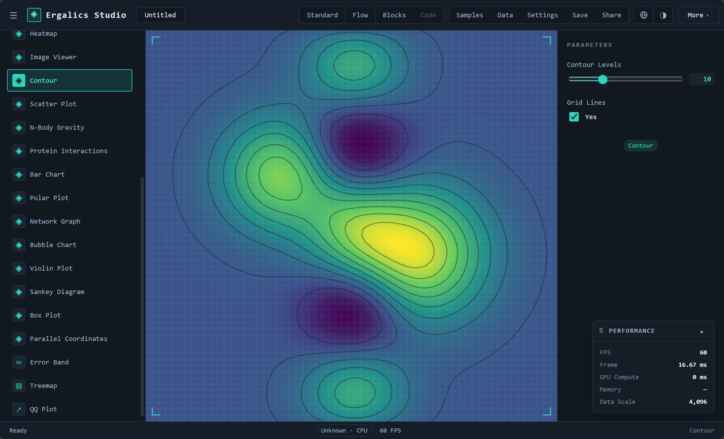
A 64×64 scalar field rendered as a viridis ramp plus marching-squares isolines — the sample twin-peak field. Demonstrates data-driven loading with the host auto-routing a .json grid to the plugin.

A 64×64 scalar-field viewer: viridis color ramp plus marching-squares isolines. Its grid normalization logic is covered by builtinPlugins.test.ts, and the bundled sample (field.json) renders the twin-peak field above.

AI Trainer (example.ai-training)

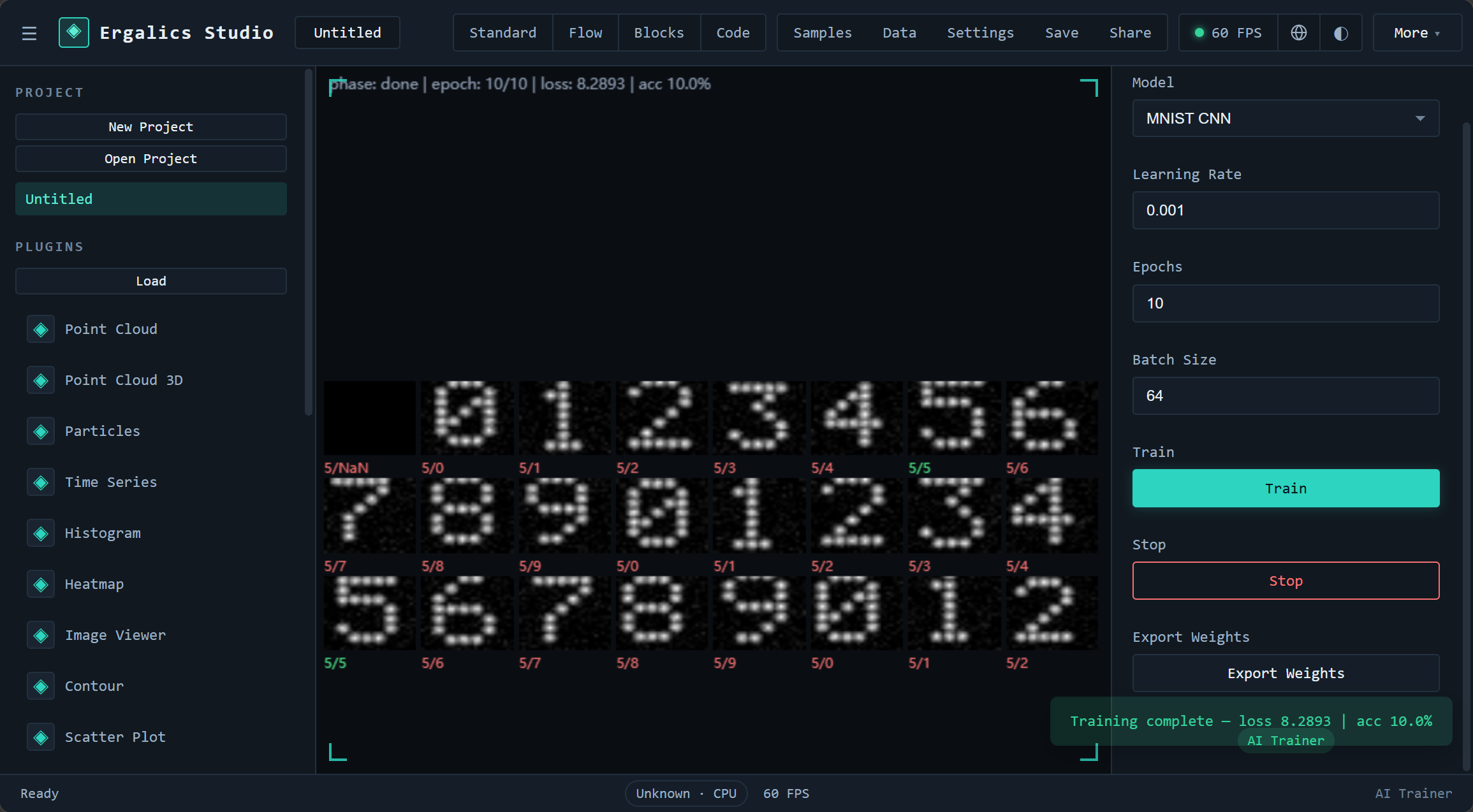
In-browser model training: the MNIST CNN grid shows prediction (green) vs. ground truth (red) per digit after 10 epochs, alongside the live-updating loss curve.

A drop-in for "train a small model in the browser without writing code". Four model kinds — linear, nonlinear-nn, logistic, mnist — share the same Train / Stop / Export Weights button surface and the same live-updating loss curve. A handy reference for plugin authors because it exercises several host features at once:

• loadData(file) parses tabular CSV through a single helper and accepts the MNIST 785-column label,p0..p783 layout. The host router picks the right plugin from the file's extension, so dropping a CSV onto the canvas is enough to start training.
• button parameters + updateParams drive the training flow. The plugin publishes three buttons; each carries an action string (train / stop / export), and updateParams reads it back and dispatches. No custom api.* calls are required.
• A long-running compute callback streams progress via the onProgress hook so the loss curve and the lower panel repaint during training without blocking the UI.
• Dynamic imports for heavy deps. TensorFlow.js is ~2 MB and is not loaded by the auto-load step — loadTf() does await import('@tensorflow/tfjs') on first use, then prefers the WebGL backend and falls back to CPU. Plugin authors shipping a heavy native dep can follow the same pattern.
• Bundled sample data lives in examples/data/ai/ (linear, non-linear, logistic, MNIST) and is exposed through the global 示例 dialog rather than a per-plugin "Load Sample" button, so the dialog stays the single entry point for one-click data.

N-Body Gravity (example.nbody)

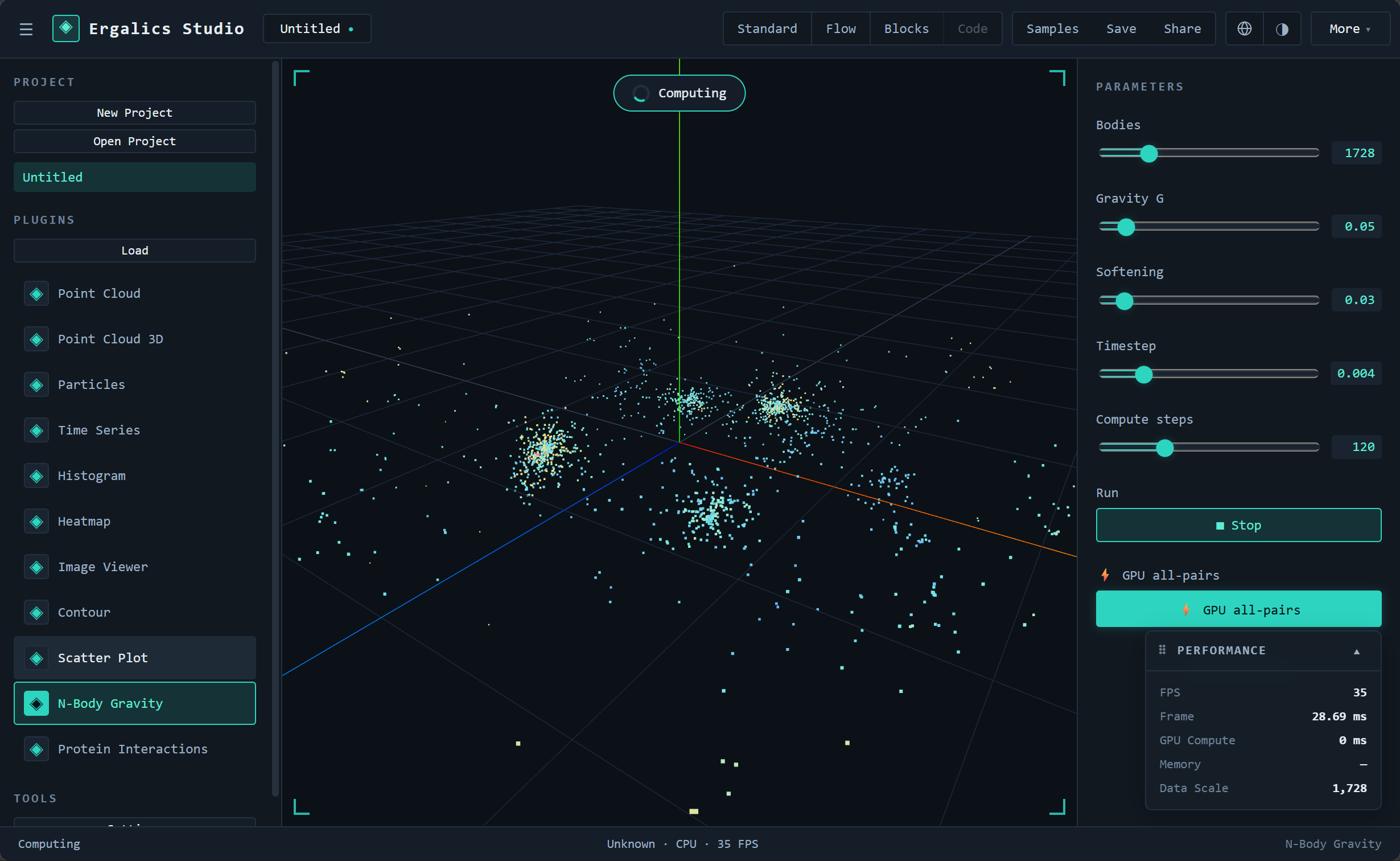
4096-body torus ring orbiting a central mass: direct-summation gravity rendered as THREE.Points via the host Three.js scene, physics advancing on the device with the WGSL all-pairs kernel.

A 3-D astrophysics demo: direct-summation gravity where every body feels the pull of every other body — O(N²) per step. It declares renderToScene, so the host materializes the Three.js scene and the plugin renders the bodies as THREE.Points (colored by speed, camera auto-fit).

• Data — JSON initial conditions. Either an array of [x, y, z, vx, vy, vz, mass] tuples or objects with those keys:

  { "bodies": [[0, 0, 0, 0, 0, 0, 50], [0.9, 0.18, 0.0, 0.01, 0, -1.56, 1]] }

  The bundled sample (nbody.json) is a 4096-body torus ring orbiting a central mass.
• Compute — the GPU all-pairs button (or compute()) uploads the bodies to an interleaved [x,y,z,vx,vy,vz,mass] storage buffer and dispatches a WGSL all-pairs kernel. Two buffers are used in ping-pong so every integration step stays on the device with no per-step read-back. On CPUs (or when api.gpu is absent) the identical integrator (advanceNBodyCPU in src/core/wgsl.ts) runs as a fallback.
• Parameters — Bodies (resample count), Gravity G, Softening, Timestep, Compute steps, a Run toggle (live animation), and the GPU compute button.
• The plugin is data-driven: it renders an empty scene until a .json file or sample data is loaded, and it never fabricates a dataset.

Protein Interactions (example.protein)

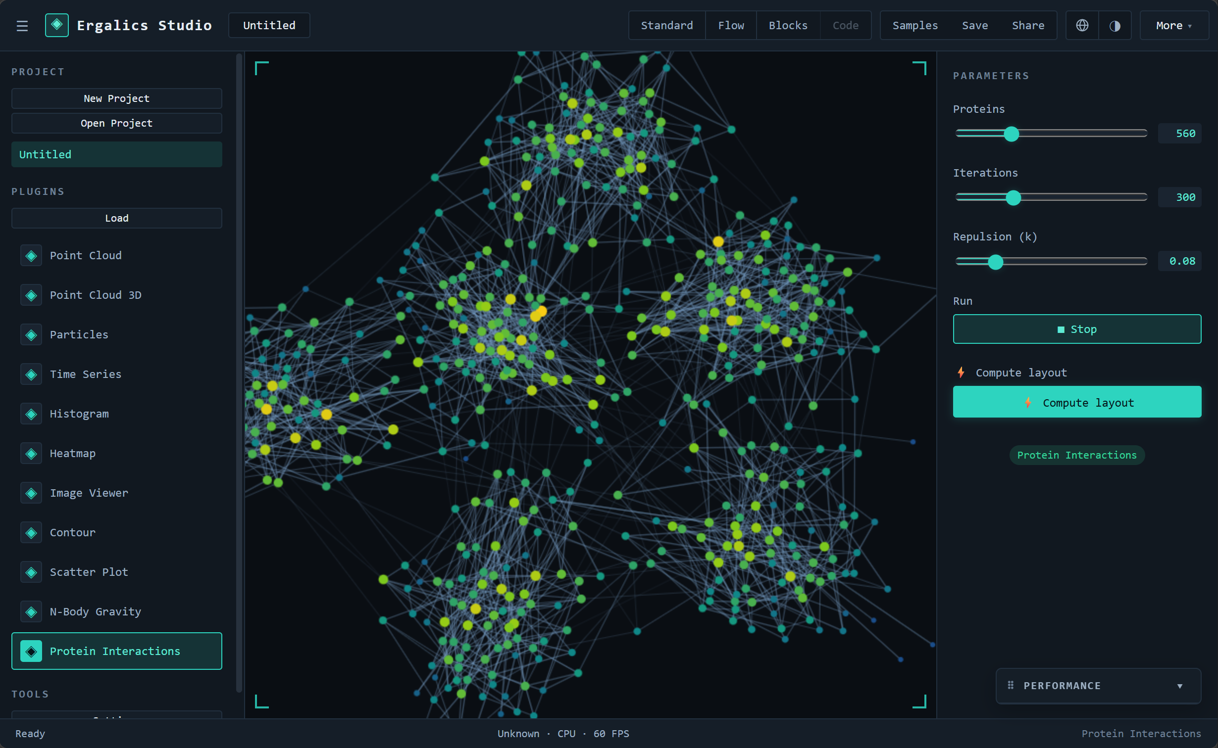
Force-directed (Fruchterman-Reingold) layout of the 560-protein PPI network, nodes colored and sized by degree; the layout anneals to convergence and reports connected components.

A systems-biology demo. Loads a protein-protein interaction (PPI) network and computes a force-directed layout (Fruchterman-Reingold spring-electrical model) — O(V²) repulsion + O(E) attraction per iteration, annealed to convergence — then reports biology-relevant metrics.

• Data — JSON with proteins ({id, name}) and interactions ({source, target, weight} or [sourceIdx, targetIdx, weight]):

  {
    "proteins": [{ "id": "P0", "name": "Protein-0" }],
    "interactions": [{ "source": "P0", "target": "P1", "weight": 0.8 }]
  }

  The bundled sample (protein.json) is a 560-protein / ~1700-interaction modular network.
• Compute — the Compute layout button runs Iterations steps of the layout with simulated-annealing temperature decay, then reports the number of connected components (putative complexes/modules) and the largest component size via the ComputeResult.output.
• Parameters — Proteins, Iterations, Repulsion (k), a Run toggle (live relaxation), and the compute button. The live animation anneals its temperature and auto-stops once settled, so nodes do not jitter.
• Nodes are colored by degree and sized by degree; edges are weighted.

LBM Fluid (example.fluid)

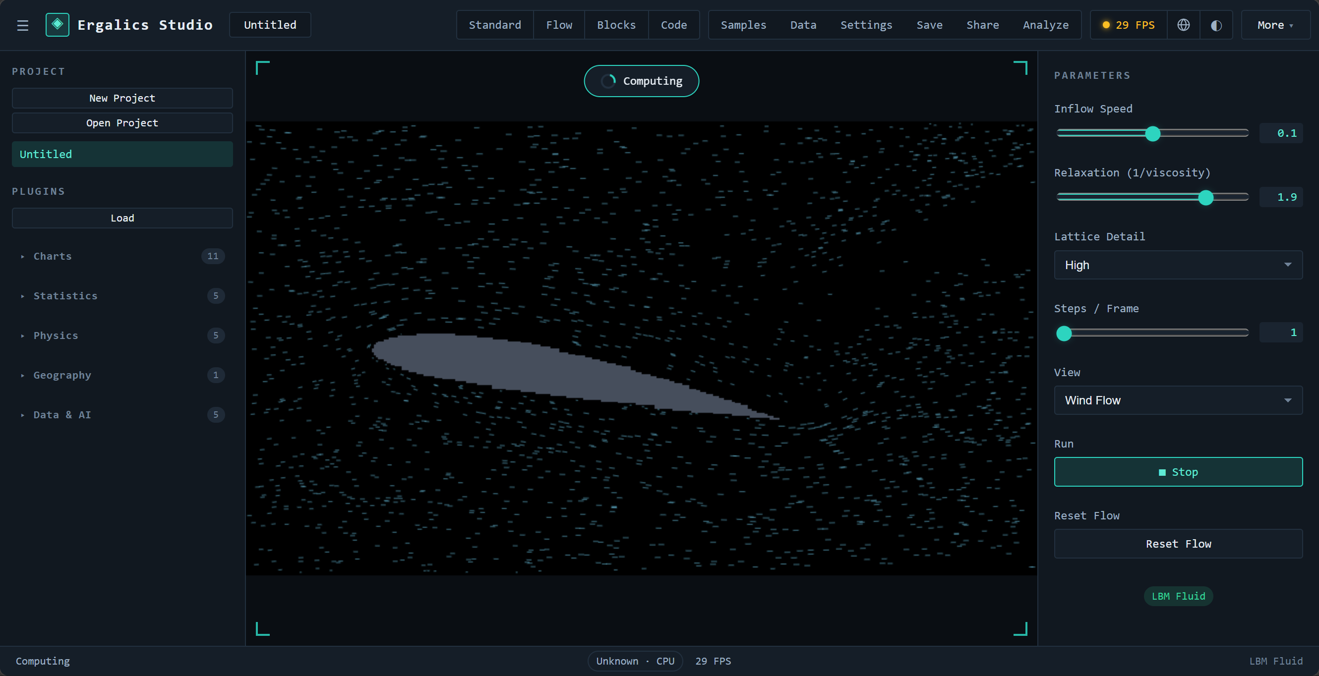
Lattice-Boltzmann (D2Q9) channel flow past an airfoil mask in the Wind Flow view; collide and stream run as WGSL kernels and develop a Kármán vortex street.

A 2-D lattice-Boltzmann channel flow (D2Q9) around a user-supplied obstacle mask. Collide and stream steps run as WGSL kernels (with a matching fluidStepCPU fallback pinned by tests), and long obstacles develop a Kármán vortex street.

• Data — JSON obstacle mask where 1 marks solid cells. The bundled sample (fluid-obstacle.json) is an airfoil profile.
• Parameters — Inflow Speed, Relaxation (1/viscosity), Lattice Detail, Steps / Frame, a View selector (Wind Flow / vorticity and friends), plus Run / Stop and Reset Flow.
• Like every simulation plugin it is strictly data-driven: it starts empty and never fabricates a default scene.

Wave Equation (example.wave)

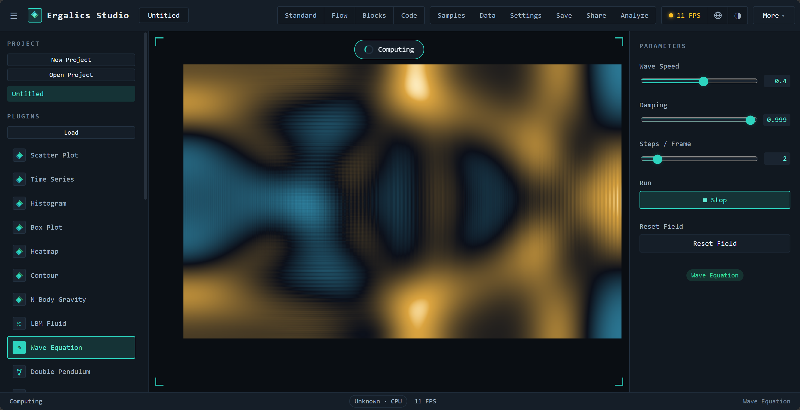
2-D finite-difference wave equation (leapfrog WGSL kernel): the twin-source sample shows two circular waves interfering into the characteristic orange/blue amplitude lattice.

A 2-D finite-difference wave equation on a grid, integrated by a WGSL leapfrog kernel (waveStepCPU as tested CPU fallback).

• Data — JSON with a u grid and an optional drive grid (< 0 barrier, > 0 source amplitude). Three bundled samples cover the scenarios: wave-pulse.json, wave-twin.json (two-source interference), and wave-slit.json (double slit).
• Parameters — Wave Speed, Damping, Steps / Frame, Run/Stop, and Reset Field.

Double Pendulum (example.pendulum)

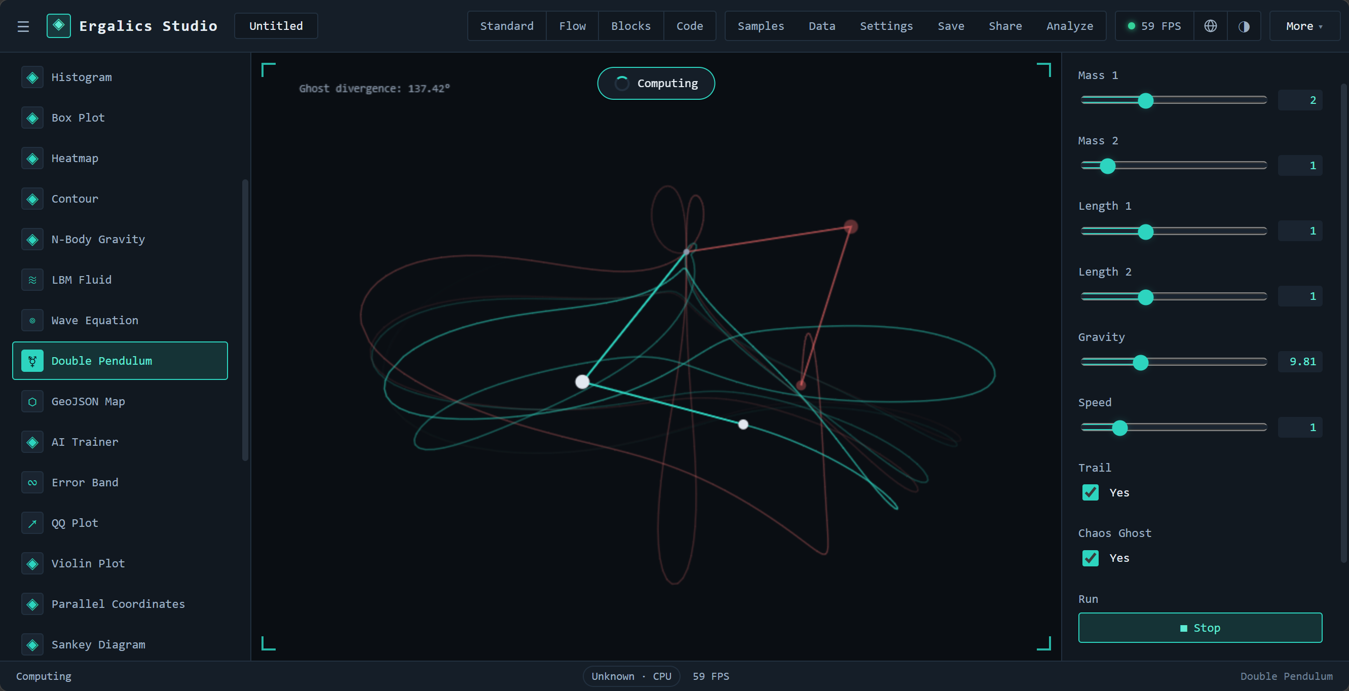
Two RK4-integrated double pendulums whose initial angles differ by only 0.001 rad; the HUD shows the live ghost divergence (137.42°) as the trajectories peel apart — a direct visual of chaos.

A chaos demonstration: two double pendulums integrated with RK4, the ghost twin starting at an angle offset of just 0.001 rad. The HUD reads out the live ghost divergence so sensitive dependence on initial conditions is directly visible as the trajectories peel apart.

• Data — JSON initial conditions (angles + angular velocities). Bundled samples: pendulum-chaos.json and pendulum-flip.json.
• Parameters — Mass 1/2, Length 1/2, Gravity, Speed, a trail toggle, the Chaos Ghost toggle, and Run/Stop.

GeoJSON Map (example.geomap)

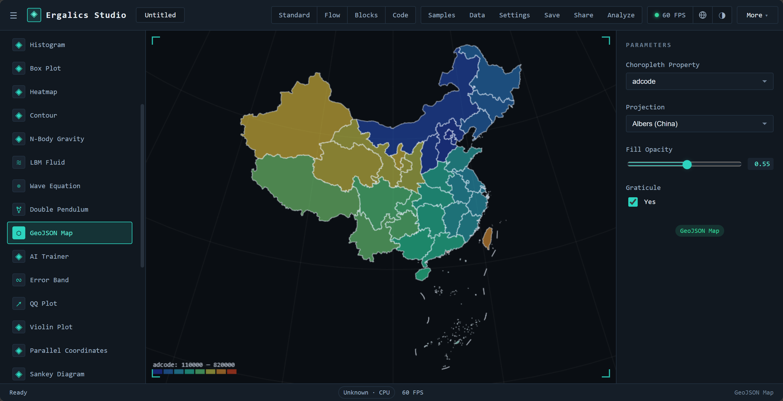
Offline GeoJSON choropleth of China's provinces shaded by a property in the Albers (China) projection — no tile server, no network.

An offline vector map: loads a GeoJSON FeatureCollection and shades each feature by a chosen property (choropleth) — no tile server, no network.

• Data — .geojson (or .json) files. Bundled samples: china-provinces.geojson (province polygons with adcode) and choropleth-sample.geojson.
• Parameters — Choropleth Property, Projection (Albers (China) / Web Mercator / equirectangular), Fill Opacity, and a graticule toggle.
• parseGeoJSON — geometry and property extraction — is unit-tested in geoPhysicsPlugins.test.ts alongside the fluid / wave / pendulum logic.

All built-ins register via BUILTIN_PLUGINS in src/plugins/builtin/index.ts and their sample data via BUILTIN_EXAMPLES in src/core/examples.ts.

Building a .cspkg package

A package is a ZIP with manifest.json + entry + assets:

my-plugin.cspkg
├── manifest.json
└── dist/
    └── index.js        # module whose default export is the plugin factory

The entry source is a function body that receives the (sandboxed) api and returns a Plugin object.

Sandboxing

• isolated (default) — the entry runs inside a Web Worker with a postMessage RPC bridge (src/core/sandbox.ts). It has no access to the host page's globals, DOM, window, or stores. Canvas rendering works via an OffscreenCanvas transferred into the worker; dom/three handles are intentionally unavailable.
• trusted — executes directly in the host context with full DOM access. Use only for packages you control.

If Workers are unavailable, the loader falls back to a best-effort strict new Function with shadowed globals and warns the user that this is not a security boundary.

Honest limits: workers share the origin's IndexedDB, so a malicious package could still read app data through it. Treat the sandbox as isolation from the page context, not from the origin's storage.